Tutorial 4: Pick particles using the general model refined for your data

With crYOLO you can train a model for your data by fine-tuning the general model.

What does fine-tuning mean?

The general model was trained on a lot of particles with a variety of shapes and therefore learned a robust set of generic features. The last layers, however, learn a fairly abstract representation of the particles and it might be that they do not perfectly fit your particle at hand. In order to adapt this abstract representation within the network to your specific particle, fine-tuning only affects the last convolutional layers, but keeps all others fixed.

Why should I fine-tune my model instead of training from scratch?

1. From theory, using fine-tuning should reduce the risk of overfitting and the amount of the required training data.

2. The training is much faster, as not all layers have to be trained.

3. The training will need less GPU memory and therefore is usable with NVIDIA cards with less memory.

Overfitting

Overfitting means, that the model works good on the training micrographs, but not on new unseen micrographs. The model just memorized what it saw instead of learning generic features.

Warning

The fine tune mode is still somewhat experimental and we will update this section as crYOLO develops over time.

If you followed the installation instructions, you now have to activate the cryolo virtual environment with

source activate cryolo

1. Data preparation

In the following I will assume that your image data is in the folder images.

The next step is to create training data. To do so, we have to pick manually in several images. Ideally, the images are picked to completion. However, it is not necessary to pick all particles. crYOLO will still converge if you miss some (or even many).

How many images have to be picked?

It depends! Typically 10 images are a good start. However, that number may increase / decrease due to several factors:

• A very heterogeneous background could make it necessary to pick more images.

• When you refine a general model, you might need to pick fewer images.

• If your micrograph is only sparsely decorated, you may need to pick more images.

We recommend that you start with 10 images, then autopick your data, check the results and finally decide whether to add more micrographs to your training set. If you refine a general model, even 5 images might be enough.

To create your training data, we developed a dedicated napari plugin called “napari-boxmanager”.

Start the box manager with the following command:

napari_boxmanager

Now press File -> Open Folder and the select the images directory.

Increase the contrast

You might want to run a low pass filter before you start picking to get better contrast.

1. Switch to tab bandpass_filter and check if the default LP resolution is ok and that the extracted Pixel size is correct.

2. Press Run to get a new layer with your low pass filtered images. It will filter the images on-the-fly.

Create particle layer

First you need to create a new layer for picking particles

1. Switch to the tab Organize_layer.

2. Click Create particle layer. I assume that you only have one image stack open, in case you don’t please adapt Target image layer accordingly.

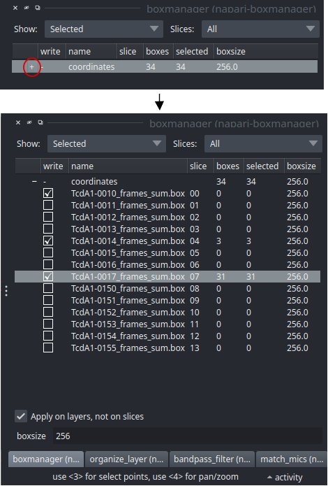
3. Switch to the boxmanager tab. Open the list of coordinates by pressing the little +. You can now navigate in the image tree and start picking.

Start picking particles

The basic usage of the boxmanager is as follows:

• Place a box: Switch the layer control (left side) to (shortcut key 2). Then you can place a box with LMB (Left mouse button).

• Move a box: Switch to the layer control to (shortcut key 3). Then you can drag a box by holding LMB.

• Delete a box: Switch the layer control to . Click on a box and press DEL

• Zoom: You can use your mouse wheel to zoom in and out.

You can change the box size in the main window, by changing the number in the text field boxsize and confirm with pressing Enter. For picking, you should the use minimum sized square which encloses your particle.

If you have images that do not contain particles but only contamination / ice you can add them to your training set by activate the checkbox in front of the image.

Save your annotations to disk

If you finished picking from your micrographs, you can export your box files in tab organize_layer. The defaults should be fine so you can directly press Save to dir. Training data is created for all micrographs that have an activated checkbox. Create a new directory called train_annotation and save it there. Close boxmanager.

Optionally, you now create a third folder with the name train_image. Now for each box file, copy the corresponding image from images into train_image.

Note

While it is nice to keep your files organized, you don’t have to copy your training images into a separate folder. In the configuration file (see below) you can also simply specify the images directory as train_image_folder. CrYOLO will find the correct images using the box files.

crYOLO will detect image / box file pairs by taking the box file and searching for an image filename which contains the box filename.

2. Start crYOLO

You can use crYOLO either by command line or by using the GUI. The GUI should be easier for most users. You can start it with:

cryolo_gui.py

The crYOLO GUI is essentially a visualization of the command line interface. On left side, you find all possible “Actions”:

• config: With this action you create the configuration file that you need to run crYOLO.

• train: This action lets you train crYOLO from scratch or refine an existing model.

• predict: If you have a (pre)trained model you can pick particles in your data set using this command.

• evaluation: This action helps you to quantify the quality of your model.

• boxmanager: This action starts the cryolo boxmanager. You can visualize the picked particles with it or create training data.

Each action has several parameters which are organized in tabs. Once you have chosen your settings you can press Start (just as example, don’t press it now ;-)), the command will be applied and crYOLO shows you the output:

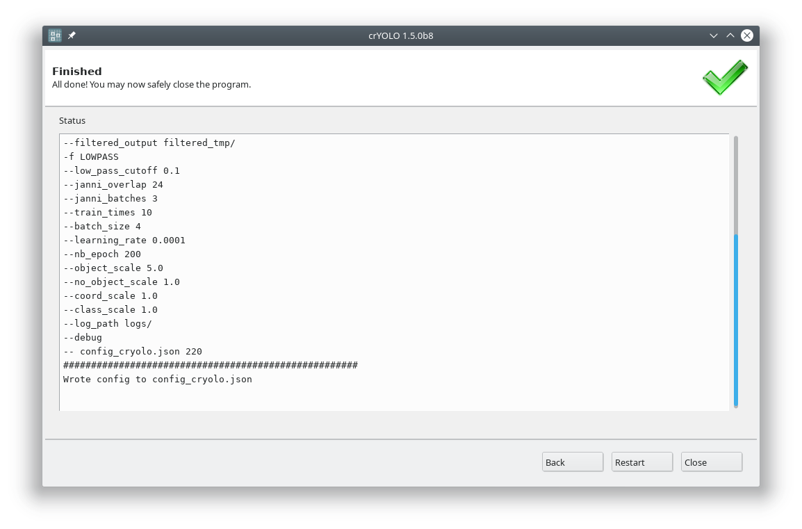
It will tell you if something went wrong. Moreover, it will tell you all parameters used. Pressing Back brings you back to your settings, where you can either edit the settings (in case something went wrong) or go to the next action.

3. Configuration

You now have to create a configuration file for your picking project. It contains all important constants and paths and helps you to reproduce your results later on.

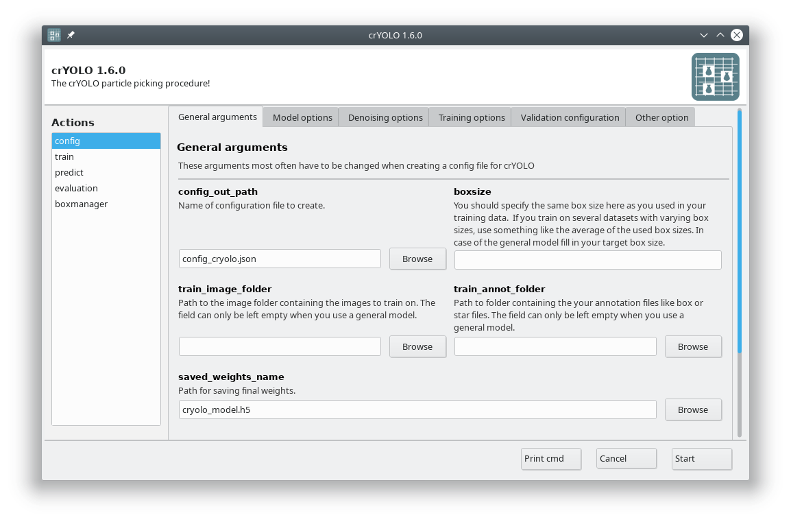
You can either use the command line to create the configuration file or the GUI. For most users, the GUI should be easier. Select the config action and fill in the general fields:

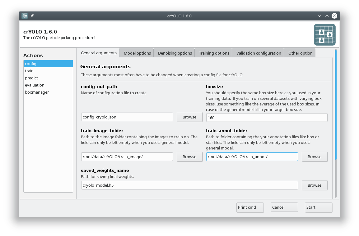
At this point you could already press Start to generate the config file but you might want to take these options into account:

Validation data

Micrographs that are selected as validation data are not used to train crYOLO. These micrographs are used to calculate how well the model performs and whether it still improves.

• During training, crYOLO also needs validation data. Typically, 20% of the training data are randomly chosen as validation data. If you want to use specific images as validation data, you can move the images and the corresponding box files to separate folders. Make sure that they are removed from the original training folder! You can then specify the new validation folders in “Validation configuration” tab.

• By default, your micrographs are low pass filtered to an absolute frequency of 0.1 and saved to disk. You can change the cutoff threshold and the directory for filtered micrographs in the “Denoising options” tab.

• When training from scratch, crYOLO is initialized with weights learned on the ImageNet training data (transfer learning). However, it might improve the training if you set the pretrained_weights options in the “Training options” tab to the current general model. Please note, doing this you don’t fine tune the network, you just change the initial model initialization.

Alternative: Using neural-network denoising with JANNI

You can also use neural network denoising with JANNI. The easiest way is to use the JANNI’s general model (Download here) but you can also train JANNI for your data. crYOLO directly uses an interface to JANNI to filter your data, you just have to change the filter argument in the Denoising tab from LOWPASS to JANNI and specify the path to your JANNI model:

I recommend to use denoising with JANNI only together with a GPU as it is rather slow (~ 1-2 seconds per micrograph on the GPU and 10 seconds per micrograph on the CPU)

Editing the configuration file

You can also modify all options and parameters directly in the config.json file. It can be opened by any text editor. Please note the wiki entry about the crYOLO configuration file if you want to know more details.

Hint

Alternative: Create the configuration file with the command line

To create a basic configuration file that will work for most projects is very simple. I assume your box files for training are in the folder train_annot and the corresponding images in train_image. I furthermore assume that your box size in your box files is 160. To create the config config_cryolo.json simply run:

cryolo_gui.py config config_cryolo.json 160 --train_image_folder train_image --train_annot_folder train_annot

To get a full description of all available options type:

cryolo_gui.py config -h

If you want to specify separate validation folders you can use the --valid_image_folder and --valid_annot_folder options:

cryolo_gui.py config config_cryolo.json 160 --train_image_folder train_image --train_annot_folder train_annot --valid_image_folder valid_img --valid_annot_folder valid_annot

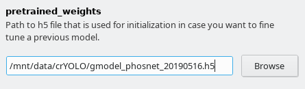
Furthermore, you have to select the model you want to refine. Download the the general model you want to refine specify in the field pretrained_weights in the Training options tab.

4. Training

Now you are ready to train the model. In case you have multiple GPUs, you should first select a free GPU. The following command will show the status of all GPUs:

>>> nvidia-smi

For this tutorial, we assume that you have either a single GPU or want to use GPU 0.

In the GUI choose the action train. In the Required arguments tab select the configuration file we created in the previous step and set the number of warmup periods to zero.

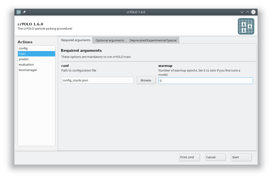
In the Optional arguments tab please check the fine_tune box.

Warning

Adjust the number of layers to train

The number of layers to fine tune (specified by layers_fine_tune in the Optional arguments tab) is still experimental. The default value of 2 worked for us but you might need more layers.

Training on CPU

The fine tune mode is especially useful if you want to train crYOLO on the CPU. On my local machine it reduced the time for training crYOLO on 14 micrographs from 12-15 hours to 4-5 hours.

You can now press the Start button to start training.

5. Picking

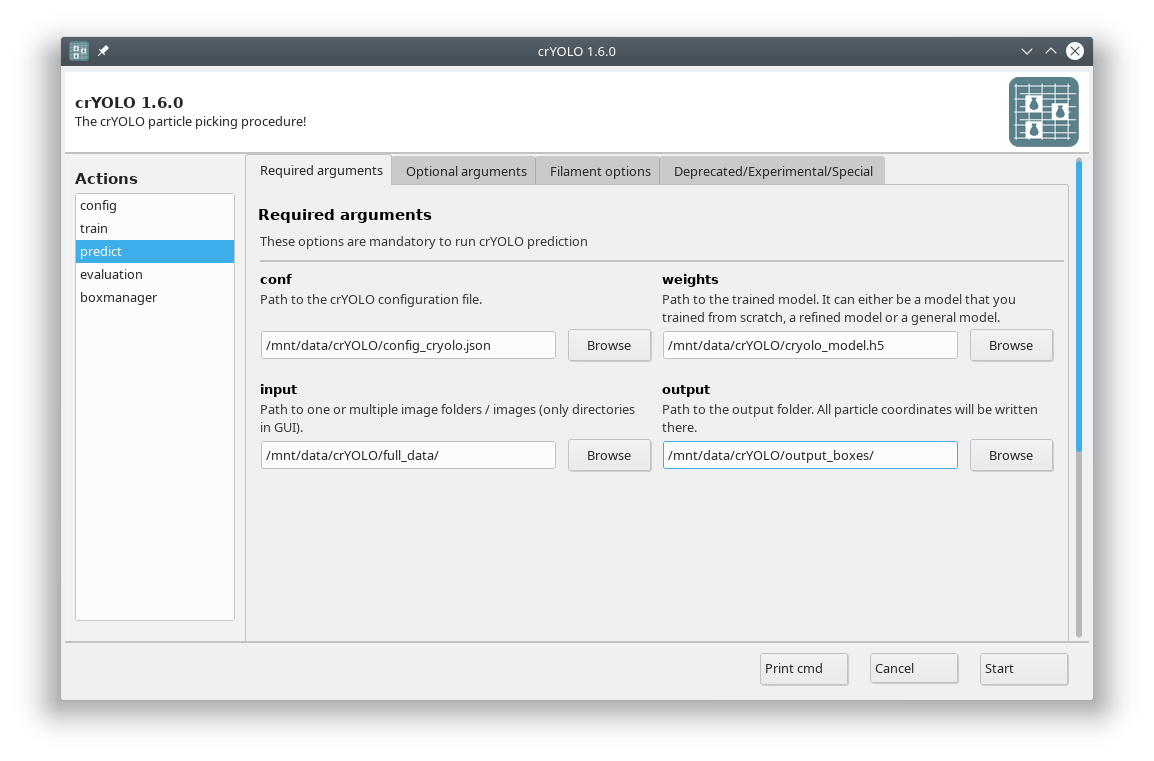
Select the action predict and fill all arguments in the Required arguments tab:

Adjusting confidence threshold

In crYOLO, all particles have an assigned confidence value. By default, all particles with a confidence value below 0.3 are discarded. If you want to pick less or more conservatively you might want to change this confidence threshold to a less (e.g. 0.2) or more (e.g. 0.4) conservative value in the Optional arguments tab. However, it is much easier to select the best threshold after picking using the CBOX files written by crYOLO as described in the next section.

crYOLO on cluster machines

Cluster machines typically use parallel filesystem, which allow the parallel reading of files. In these cases you should use more processes as cpu cores available. In GUI the you can find num_cpu under Optional arguments. On our cluster we oversubscribe a node (4 cores) by factor of 7 by setting num_cpu to 32. In the command line you can do that by using the option --num_cpu NUMBER_OF_PROCESSES.

Monitor mode

When this option is activated, crYOLO will monitor your input folder. This especially useful for automation purposes. You can stop the monitor mode by writing an empty file with the name stop.cryolo in the input directory. Just add --monitor in the command line or check the monitor box in in the Optional arguments tab

Press the the Start button to run the prediction. You can also press the Submit button to submit the job to a queueing system

After picking is done, you can find four folders in your specified output folder:

• CBOX: Contains a coordinate file in .cbox format each input micrograph. It contains all detected particles, even those with a confidence lower the selected confidence threshold. Additionally it contains the confidence and the estimated diameter for each particle. Importing those files into the boxmanager allows you advanced filtering e.g. according size or confidence.

• EMAN: Contains a coordinate file in .box format each input micrograph. Only particles with the an confidence higher then the selected (default: 0.3) are contained in those files.

• STAR: Contains a coordinate file in .star format each input micrograph. Only particles with the an confidence higher then the selected (default: 0.3) are contained in those files.

• DISTR: Contains the plots of confidence- and size-distribution. Moreover, it contains a machine readable text-file the summary statistics about these distributions and their raw data in separate text-files.

Hint

Import coordinates into Relion 4

To import your coordinates into Relion 4 a few additional steps are necessary. You find a tutorial how to do that in the “Other pages” section.

Hint

Alternative: Run prediction from the command line

To pick all your images in the directory full_data with the model weight file cryolo_model.h5 (e.g. or gmodel_phosnet_X_Y.h5 when using the general model) and and a confidence threshold of 0.3 run:

cryolo_predict.py -c config.json -w cryolo_model.h5 -i full_data/ -g 0 -o boxfiles/ -t 0.3

You will find the picked particles in the directory boxfiles.

6. Visualize the results

To visualize your results you can use the boxmanager:

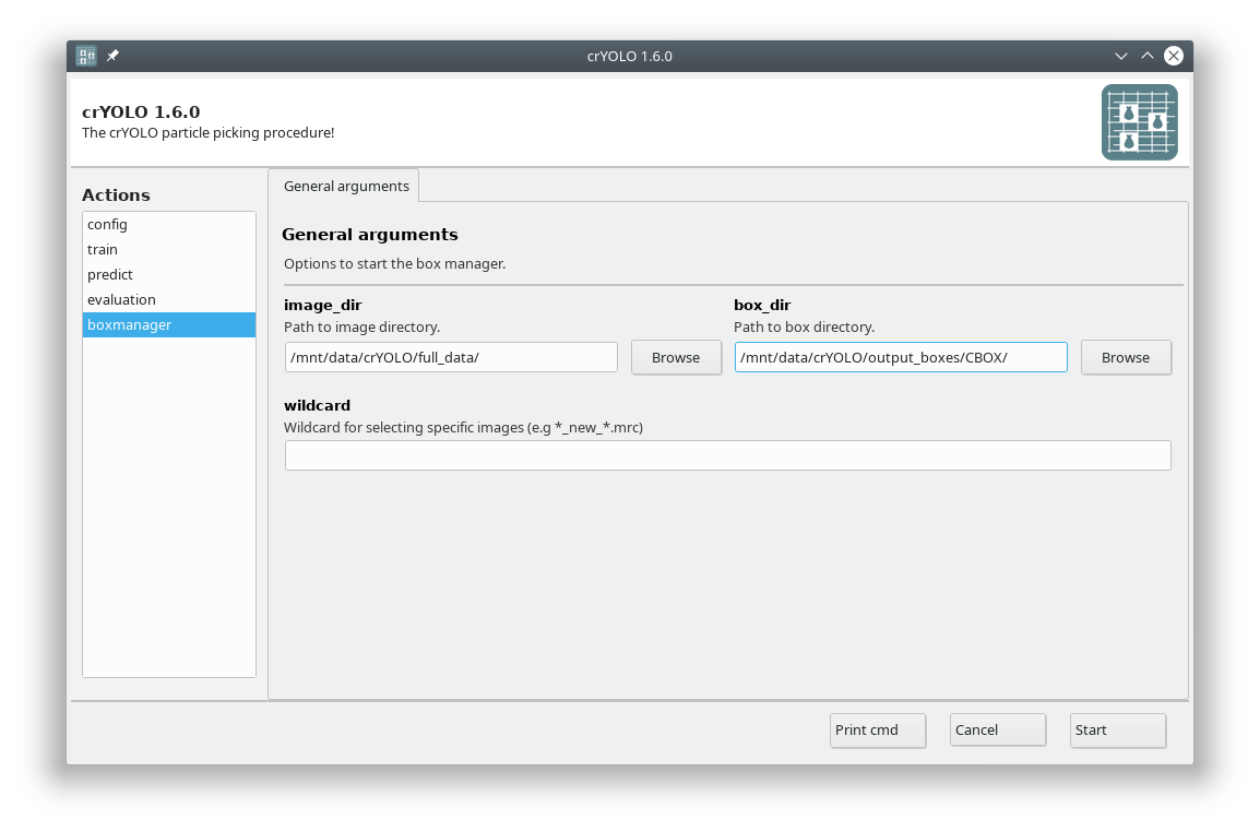
As image_dir you select the full_data directory. As box_dir you select the CBOX folder (or CBOX_FILAMENT_SEGMENTED in case of filaments).

Hint

Alternative: Open it via command line

You can also open the results via command line:

napari_boxmanager 'full_data/*.mrc' 'boxfiles/CBOX/*.cbox'

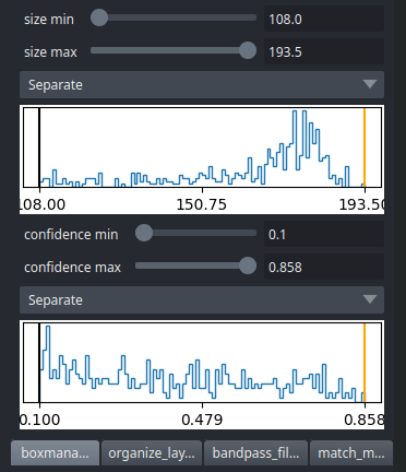
CBOX files contain besides the particle coordinates more information like the confidence and the estimated size of each particle. When importing .cbox files into the box manager, it enables more filtering options in the GUI. You can plot size- and confidence distributions. Moreover, you can change the confidence threshold, minimum and maximum size and see the results in a live preview. If you are done with the filtering, you can then write the new box selection into new box files.

7. Evaluate your results

The evaluation tool allows you, based on your validation micrographs, to get statistics about the success of your training.

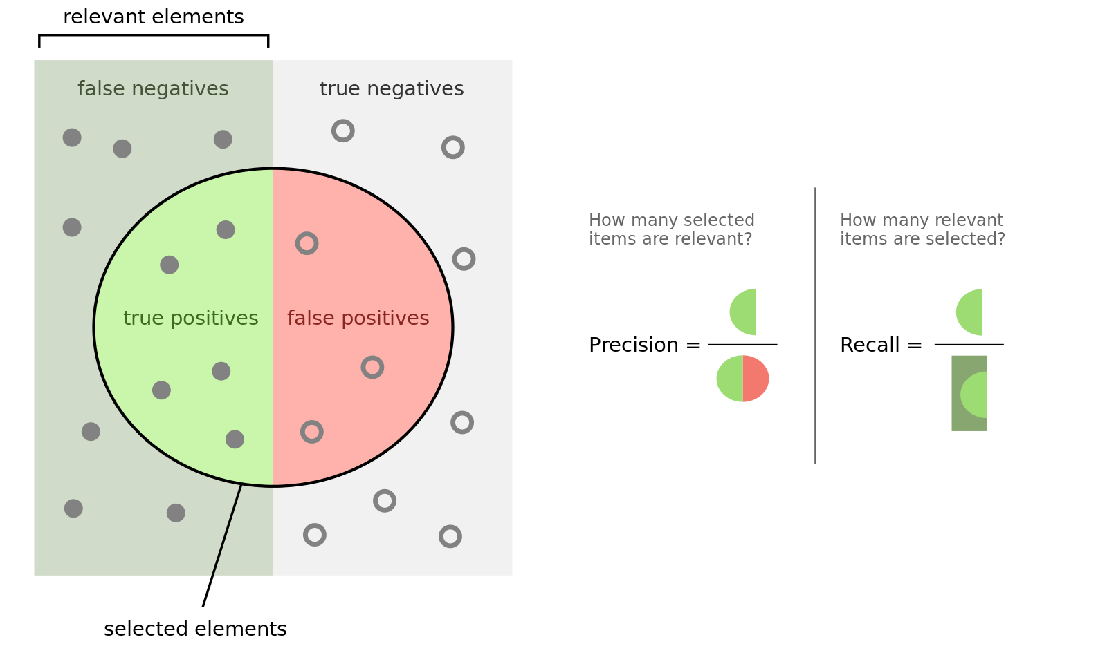
To understand the outcome, you have to know what precision and recall is. Here is good figure from wikipedia:

Another important measure is the F₁ (\(\beta = 1\)) and F₂ (\(\beta = 2\)) score:

\[F_\beta = (1+\beta)^2 \cdot \frac{precision \cdot recall}{\beta^2 \cdot precision + recall}\]

Warning

Precision metric can be misleading

If your validation micrographs are not labeled to completion the precision value will be misleading. crYOLO will start picking the remaining ‘unlabeled’ particles, but for statistics they are counted as false-positive (as the software takes your labeled data as ground truth).

If you followed the tutorial, the validation data are selected randomly. A run file for each training is created and saved into the folder logs/runfiles in your project directory. These runfiles are .json files containing information about what micrographs were selected for validation. To calculate evaluation metrics select the evaluation action.

Fill out the fields in the Required arguments tab:

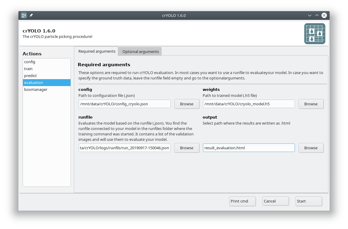
Press Start to calculate the evaluation results.

Hint

Alternative: Run evaluation from the command line

cryolo_evaluation.py -c config.json -w model.h5 -r runfiles/run_YearMonthDay-HourMinuteSecond.json -g 0

The html file you specified as output looks like this:

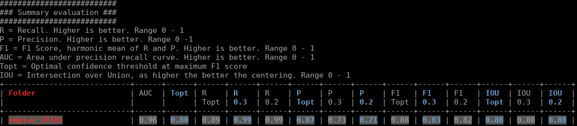
The table contains several statistics:

• AUC: Area under curve of the precision-recall curve. Overall summary statistics. Perfect classifier = 1, Worst classifier = 0

• Topt: Optimal confidence threshold with respect to the F1 score. It might not be ideal for your picking, as the F1 score weighs recall and precision equally. In single particle analysis, recall is often more important than the precision.

• R (Topt): Recall using the optimal confidence threshold.

• R (0.3): Recall using a confidence threshold of 0.3.

• R (0.2): Recall using a confidence threshold of 0.2.

• P (Topt): Precision using the optimal confidence threshold.

• P (0.3): Precision using a confidence threshold of 0.3.

• P (0.2): Precision using a confidence threshold of 0.2.

• F1 (Topt): Harmonic mean of precision and recall using the optimal confidence threshold.

• F1 (0.3): Harmonic mean of precision and recall using a confidence threshold of 0.3.

• F1 (0.2): Harmonic mean of precision and recall using a confidence threshold of 0.2.

• IOU (Topt): Intersection over union of the auto-picked particles and the corresponding ground-truth boxes. The higher, the better – evaluated with the optimal confidence threshold.

• IOU (0.3): Intersection over union of the auto-picked particles and the corresponding ground-truth boxes. The higher, the better – evaluated with a confidence threshold of 0.3.

• IOU (0.2): Intersection over union of the auto-picked particles and the corresponding ground-truth boxes. The higher, the better – evaluated with a confidence threshold of 0.2.

If the training data consist of multiple folders, then evaluation will be done for each folder separately. Furthermore, crYOLO estimates the optimal picking threshold regarding the F₁ Score and F₂ Score. Both are basically average values of the recall and prediction, whereas the F₂ score puts more weights on the recall, which is in cryo-EM often more important.